
How a molecular structure becomes a spectrum — and what to check before comparing it with your measurement.
Can a high-field reference help with your benchtop spectrum?
A high-field reference can help you assess a benchtop spectrum when suitable parameters and sample conditions support the comparison. Parameter determination and field-dependent spin simulation are separate steps. Neither a rescaled spectrum nor a field conversion alone establishes sample identity.
You have reference data at 400 MHz and measure the same compound on a benchtop instrument at 80 MHz. Can you compare both when the multiplets look different?
Yes, the comparison can be useful. But you should not expect a high-field reference spectrum to become a valid benchtop spectrum through simple rescaling alone.
The comparison needs more than similar lines.
Which chemical shifts and couplings define the spin system behind the comparison? Under which conditions were they determined? And how does the pattern at your field follow from them?
Referencing, solvent, temperature, pH and concentration can affect the comparison. They belong to the conditions under which the parameters apply.
Splitting the route into two steps helps: first determine the parameters, then calculate the spin system for the chosen field.
That separation does not tell you whether your sample has the expected structure. It shows which assumptions you test when calculation and measurement agree, or when they do not.
First, establish the parameters
A drawn structure contains no ready-made list of shifts δ and couplings J. These values must be determined: from experimental reference data, statistical prediction or quantum-chemical calculation, also in combination.
DFT can provide isotropic magnetic shieldings and scalar spin-spin coupling constants. Chemical shifts are derived from the shieldings by suitable referencing. Functional, basis set and referencing therefore belong to the result. [1]
For a flexible molecule, a further question arises: which arrangements are relevant under the conditions considered?
One optimised geometry is not automatically an adequate description of your solution. Conformer search and weighting must justify the arrangements considered.
Population-weighted averaging presupposes fast exchange on the NMR timescale, relative to the frequency difference of the exchanging signals. In slow or intermediate exchange, separate states or exchange lineshapes are needed, for example with slow tautomerisation or protonation. Solid-state NMR follows other conditions. [4]
The origin of a δ value is therefore not the only interesting point. You also want to know which structure, state and environment it describes.
That sounds like much accompanying information for one curve. It is exactly what later helps you place a deviation: does it come from the structural assumption, the parameters or the conditions?
Calculated parameters are neither measured values nor arbitrary estimates. They are results of a method with nameable prerequisites. Which matter in your case is what the check must show.
Then calculate the spin system
The second step begins. Shifts and couplings describe the spin system, and from them the expected spectrum is calculated. The spin Hamiltonian used captures the contributions relevant to the solution spectrum, in particular chemical shifts and scalar couplings.
The external magnetic field, equivalently the spectrometer frequency, is an input to this calculation. It is not a label added afterwards beneath the finished curve.
What matters for the line pattern is the size of the frequency differences in Hz from the shifts relative to the coupling constants. This ratio depends on field strength. [1] [2]
Presenting the lines also requires assumptions, for instance about linewidth. A convincing overlay does not show that all underlying parameters are correct.
With a suitable, assigned set of δ and J values you can calculate the expected spectrum for another field strength, provided the states and sample conditions are comparable. A reference spectrum supplied as a curve does not provide these inputs completely or unambiguously. Spin simulation does not repair incorrect inputs.
The parameters need not come from DFT. Experimentally determined values can serve as a basis. What matters is disclosing their origin and not confusing parameter determination with the calculation of the line pattern.
A new curve is therefore not new evidence. It is the consequence of the chosen inputs.
What changes between 80 and 400 MHz?
Why does the pattern change at all?
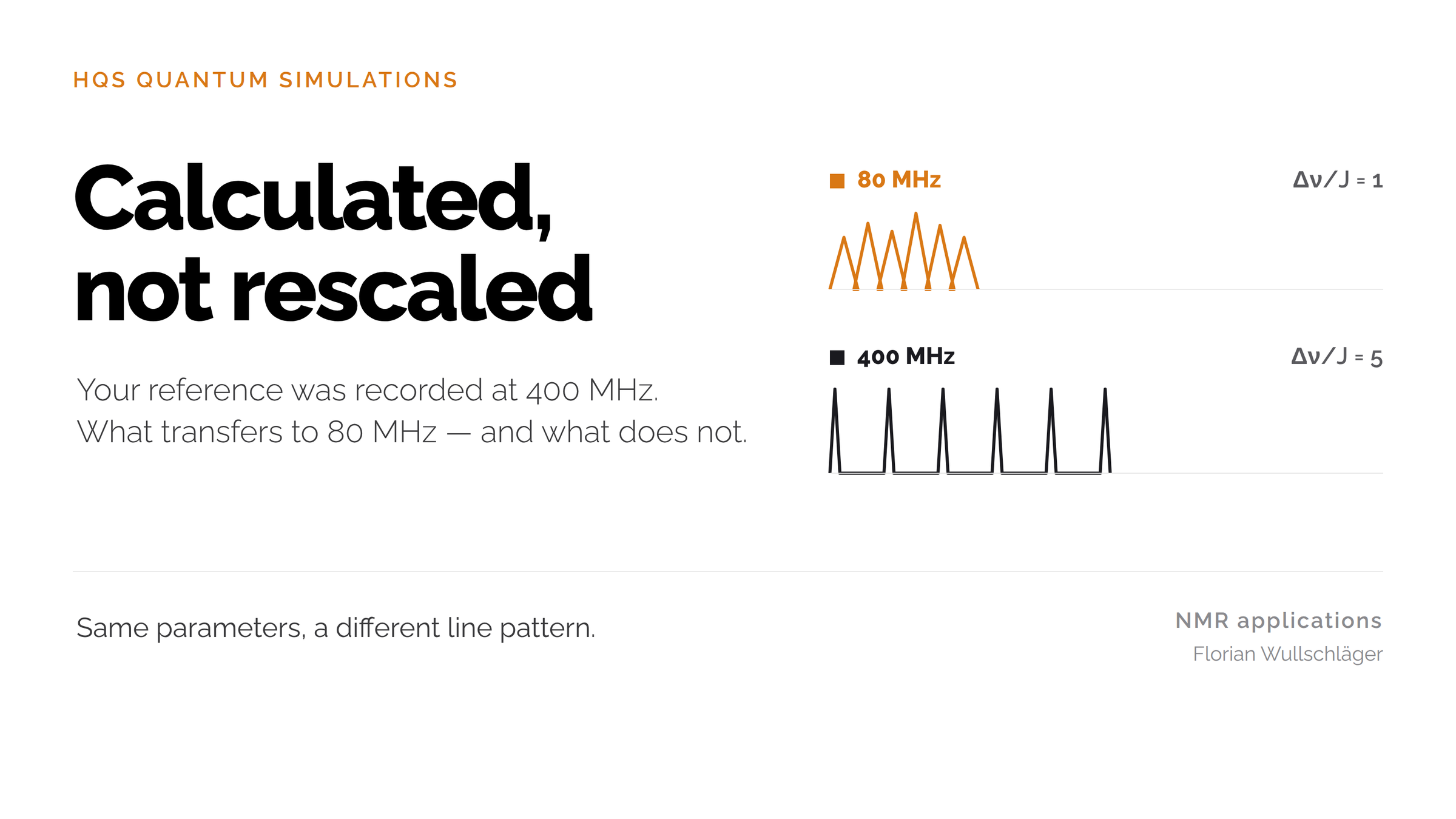
For the same underlying spin system under otherwise comparable conditions, the chemical-shift difference in ppm remains approximately constant. In Hz it grows with spectrometer frequency. The scalar coupling J in Hz remains independent of the external field. [2] [3]
A simplified two-proton model makes this tangible: a shift difference of 0.10 ppm and a coupling of 8 Hz.
At 80 MHz, 0.10 ppm corresponds to a frequency difference of 8 Hz. At 400 MHz it is 40 Hz. The ratio Δν/J rises from 1 to 5.
At the smaller (Δν/J) ratio, the coupling contributes more strongly relative to the frequency separation. Second-order effects can become more pronounced. This includes roofing: relative line intensities can become asymmetric, so that coupled multiplets appear tilted towards one another. [2] [3]
At 400 MHz these effects can be weaker. They do not disappear automatically. A high-field spectrum is not necessarily first order either.
No blanket assessment of your benchtop instrument follows. The question is which information the pattern carries for your task and whether the calculation describes it under suitable assumptions.
You are not comparing two identical curves. You are checking whether one consistent spin system explains both field strengths. That is more informative than treating an unfamiliar multiplet as a contradiction.
Uncertainty ranges first, then fit to the measurement
A quantum-chemical prediction supplies more than starting values. For comparison with a measurement these values need justified uncertainty ranges: how far may a parameter deviate before it no longer fits the prediction?
These ranges are set before the fit, for example in the range of 0.2 or 0.3 ppm for chemical shifts, depending on the method and application range. They must not be derived from the desired agreement.
Then fitting begins. The solver calculates a spectrum from the starting parameters and compares it with the measurement. Shifts and couplings are adjusted and the solver runs again to reduce the remaining difference. Which parameters may change, and when optimisation ends, is defined in advance. [5]
The result is examined on two levels: how well does the fitted spectrum describe the measurement, and how far did the parameters move from the prediction?
Changes within the defined ranges are consistent with the prediction to that extent. If parameters must move beyond them, a good curve fit does not explain the contradiction. Then check assignment, sample conditions, conformer description or prediction method.
With correlated uncertainties, individual ranges in isolation are not enough. Residual deviations and the uniqueness of the fit matter as well. Different parameter sets can produce a very similar fit, particularly when parameters are correlated. [5]
This names the limit. The calculation can show whether a model explains the measurement under the chosen assumptions. It does not prove a structure and replaces neither an independent assignment nor a validation for your purpose. Accuracy depends on input parameters and conditions, not on the number of iterations.
Are the fitted changes consistent with the prediction?
This turns a comparison of curves into a concrete check of prediction and adjustment. Three questions help.
1. What do the uncertainty ranges rest on? Document starting values, method and sample conditions, and the basis and meaning of the ranges. Record whether they describe individual parameters or a joint range.
2. What was the fit allowed to change? Define variable parameters, limits and stopping criteria. Document shifts and couplings separately from settings such as linewidth or a referencing offset. Check which regions remain unexplained.
3. Are the necessary changes consistent with the prediction? Compare starting and fitted values with the ranges defined beforehand. A good fit is not enough if implausible parameter changes were required.
Document the original prediction, the uncertainty ranges, the fitted parameters and the remaining spectral deviations side by side. Then it is traceable what was predicted and what was adjusted.
Spin simulation calculates the line pattern from the entered chemical shifts and couplings at the chosen field strength. Depending on the model, further assumptions enter the representation, for instance linewidth, populations or exchange processes. Comparing fitted values with the ranges shows whether the adjustment is consistent with the prediction.
Which difference are you trying to explain?
Back at 80 MHz, a different multiplet is not counter-evidence against the reference or against a structure derived from it. It is a reason to look at parameters, field dependence and conditions separately.
Which deviation is holding you up: the position of a signal, its splitting, or the ratio of line intensities?
If you want to discuss the comparison, write to me. The question, both field strengths and the sample conditions are a useful start. Confidential structures and data do not belong in public comments.
Then we can clarify what is comparable, which details are missing and which check makes sense next. Whether this leads to a robust decision depends on the case.
Sources
[1] ORCA Manual, §5.21: NMR Parameters. Shielding, referencing, coupling calculations, and the separate simulation step. This describes a general method, not the implementation of HQSpectrum.
[2] William Reusch, NMR Spectroscopy: Additional Information. Sections on spin-spin coupling, magnetic field strength, and hydrogen bonding.
[3] ACD/Labs, ¹H–¹H Coupling in Proton NMR, 21 August 2025. Coupling constants and second-order effects.
[4] Kleckner and Foster, An introduction to NMR-based approaches for measuring protein dynamics, §2.2. General exchange regimes and population-weighted chemical shifts; not evidence for a specific HQS conformer model.
[5] Quantum Mechanical NMR Full Spin Analysis in Pharmaceutical Identity Testing and Quality Control, §§4.1–4.3 and 5.4. Iterative adjustment and fit ambiguity; not a source for specific HQS prediction intervals.